R Time Series Objects vs Data Frames: Advantages and Limitations

As I learn more and more about R, questions often arise about which packages/methods/tools to use for a given situation. R is a vast - and growing - universe and I’m not interested in learning everything in that universe. I’m interested in learning the shortest paths between where I am now and my objective. As an adherent of the tidyverse, I lean strongly toward solutions in that realm. But, to paraphrase an old saying, ‘tidyverse is a playgound…not a jail’ and if a problem can be handled better by stepping outside the tidyverse, I’m all for that.

One of these areas is in dealing with time series: data sets comprised of repeated measurements over consistent time intervals (hourly, daily, monthly, etc). You can work with time series data using data frames, the fundamental building block of data analysis in R, but there are more specialized tools that offer more flexibility, specific capabilities and ease of use when analyzing time-based data. This can come into play in a wide variety of situations: weekly website visits, monthly sales, daily stock prices, annual GDP, electricity use by minute, that kind of thing.

So what are these time series advantages? How do we leverage them? What limitations of time series objects are good to be aware of? I’m not pretending this is a definitive guide, but I’ve been looking at this for a while and hear are my observations…

(A word on forecasting: this is a MAJOR use case for time series but is not the main focus here and I’ll only touch on that briefly below.)

Time Series Essentials

ts is the basic class for time series objects in R. You can do a lot with ts but its functionality have been extend by other packages, in particular zoo and more recently xts.

xts is a leading, evolved R package for working with time series. It builds on zoo, an earlier pkg for handling time series in R. Datacamp has a very nice

So I’m just going to scratch the surface and hit some highlights with examples here.

Get a Time Series Object

At its most basic, a time series object is a list or sometimes matrix of observations at regular time intervals.

Examples in built-in R data sets include:

• annual Nile river flows

class(Nile)

[1] "ts"

str(Nile)

 Time-Series [1:100] from 1871 to 1970: 1120 1160 963 1210 1160 1160 813 1230 1370 1140 ...

Nile

Time Series:
Start = 1871 
End = 1970 
Frequency = 1 
  [1] 1120 1160  963 1210 1160 1160  813 1230 1370 1140  995  935 1110  994 1020
 [16]  960 1180  799  958 1140 1100 1210 1150 1250 1260 1220 1030 1100  774  840
 [31]  874  694  940  833  701  916  692 1020 1050  969  831  726  456  824  702
 [46] 1120 1100  832  764  821  768  845  864  862  698  845  744  796 1040  759
 [61]  781  865  845  944  984  897  822 1010  771  676  649  846  812  742  801
 [76] 1040  860  874  848  890  744  749  838 1050  918  986  797  923  975  815
 [91] 1020  906  901 1170  912  746  919  718  714  740

• monthly Air Passengers - yes, I know everybody uses Air Passengers for their time series example. So damn handy. Different examples below, I promise. ;)

class(AirPassengers)

[1] "ts"

str(AirPassengers)

 Time-Series [1:144] from 1949 to 1961: 112 118 132 129 121 135 148 148 136 119 ...

AirPassengers

     Jan Feb Mar Apr May Jun Jul Aug Sep Oct Nov Dec
1949 112 118 132 129 121 135 148 148 136 119 104 118
1950 115 126 141 135 125 149 170 170 158 133 114 140
1951 145 150 178 163 172 178 199 199 184 162 146 166
1952 171 180 193 181 183 218 230 242 209 191 172 194
1953 196 196 236 235 229 243 264 272 237 211 180 201
1954 204 188 235 227 234 264 302 293 259 229 203 229
1955 242 233 267 269 270 315 364 347 312 274 237 278
1956 284 277 317 313 318 374 413 405 355 306 271 306
1957 315 301 356 348 355 422 465 467 404 347 305 336
1958 340 318 362 348 363 435 491 505 404 359 310 337
1959 360 342 406 396 420 472 548 559 463 407 362 405
1960 417 391 419 461 472 535 622 606 508 461 390 432

Both these examples are time series of the ts class, and we can see right off that these are different data structures from data frames. A key thing to note about time series is that date/time is not in a column the way it would be in a data frame, but is in an index - similar to row.names in a data frame.

If we look at the index for the Nile river data, we can see the time values and we can check the start and end. This info corresponds to the structure info shown above, where start = 1871, end = 1970, and frequency = 1, meaning 1 observation per year, annual data.

index(Nile)

  [1] 1871 1872 1873 1874 1875 1876 1877 1878 1879 1880 1881 1882 1883 1884 1885
 [16] 1886 1887 1888 1889 1890 1891 1892 1893 1894 1895 1896 1897 1898 1899 1900
 [31] 1901 1902 1903 1904 1905 1906 1907 1908 1909 1910 1911 1912 1913 1914 1915
 [46] 1916 1917 1918 1919 1920 1921 1922 1923 1924 1925 1926 1927 1928 1929 1930
 [61] 1931 1932 1933 1934 1935 1936 1937 1938 1939 1940 1941 1942 1943 1944 1945
 [76] 1946 1947 1948 1949 1950 1951 1952 1953 1954 1955 1956 1957 1958 1959 1960
 [91] 1961 1962 1963 1964 1965 1966 1967 1968 1969 1970

start(Nile)

[1] 1871    1

end(Nile)

[1] 1970    1

As discussed above, ts is useful, but xts offers additional flexibility and features.

Convert ts to xts

Converting to an xts object can often make the data more intuitive to deal with.

library(xts)
Nile_xts <- as.xts(Nile)
str(Nile_xts)

An xts object on 1871-01-01 / 1970-01-01 containing: 
  Data:    double [100, 1]
  Index:   Date [100] (TZ: "UTC")

head(Nile_xts)

           [,1]
1871-01-01 1120
1872-01-01 1160
1873-01-01  963
1874-01-01 1210
1875-01-01 1160
1876-01-01 1160

Air_xts <- as.xts(AirPassengers)
str(Air_xts)

An xts object on Jan 1949 / Dec 1960 containing: 
  Data:    double [144, 1]
  Index:   yearmon [144] (TZ: "UTC")

head(Air_xts)

         [,1]
Jan 1949  112
Feb 1949  118
Mar 1949  132
Apr 1949  129
May 1949  121
Jun 1949  135

• We can see here that xts has reshaped the data from a matrix with rows by year and columns by month to more ‘tidy’ data with mth-year as index and observations in one column.

Native xts

Some data comes as xts time series out of the box. For example, the quantmod package fetches stock market data as xts time series automatically:

library(quantmod)
## use quantmod pkg to get some stock prices as time series
price <- getSymbols(Symbols='EA', from="2020-01-01", to=Sys.Date(), auto.assign=FALSE)
class(price)

[1] "xts" "zoo"

head(price)

           EA.Open EA.High EA.Low EA.Close EA.Volume EA.Adjusted
2020-01-02     108     108    107      107   1901000         106
2020-01-03     106     108    105      107   1840300         106
2020-01-06     107     109    107      109   2934200         107
2020-01-07     109     109    108      108   1692400         107
2020-01-08     108     110    108      109   2651600         108
2020-01-09     110     110    108      109   1818600         108

As noted, a key characteristic of time series object is that dates are in an index rather than being in a date column, as they would be in typical data frame. Looking at the structure of the xts object, we can again see it is different from a data frame.

str(price)

An xts object on 2020-01-02 / 2023-04-06 containing: 
  Data:    double [822, 6]
  Columns: EA.Open, EA.High, EA.Low, EA.Close, EA.Volume ... with 1 more column
  Index:   Date [822] (TZ: "UTC")
  xts Attributes:
    $ src    : chr "yahoo"
    $ updated: POSIXct[1:1], format: "2023-04-08 16:50:35"

Convert xts to data frame

If you want to work with the time series as a data frame, it is fairly straightforward to convert an xts object:

price_df <- as.data.frame(price)
## add Date field based on index (row names) of xts object
price_df$Date <- index(price)
## set data frame row names to numbers instead of dates
rownames(price_df) <- seq(1:nrow(price))
## reorder columns to put Date first
price_df <- price_df %>% select(Date, 1:ncol(price_df)-1)
## check out structure using glimpse, as is the fashion of the times
glimpse(price_df)

Rows: 822
Columns: 7
$ Date        <date> 2020-01-02, 2020-01-03, 2020-01-06, 2020-01-07, 2020-01-0…
$ EA.Open     <dbl> 108, 106, 107, 109, 108, 110, 109, 109, 110, 110, 110, 112…
$ EA.High     <dbl> 108, 108, 109, 109, 110, 110, 109, 110, 110, 110, 111, 113…
$ EA.Low      <dbl> 107, 105, 107, 108, 108, 108, 108, 109, 109, 109, 110, 112…
$ EA.Close    <dbl> 107, 107, 109, 108, 109, 109, 109, 110, 110, 110, 111, 113…
$ EA.Volume   <dbl> 1901000, 1840300, 2934200, 1692400, 2651600, 1818600, 1756…
$ EA.Adjusted <dbl> 106, 106, 107, 107, 108, 108, 107, 108, 108, 108, 110, 111…

Data frame is basically a straight-up table, whereas the xts object has other structural features.

Convert data frame to xts

## convert data frame to xts object by specifying the date field to use for xts index.
price_xts <- xts(price_df, order.by=as.Date(price_df$Date))
str(price_xts)

An xts object on 2020-01-02 / 2023-04-06 containing: 
  Data:    character [822, 7]
  Columns: Date, EA.Open, EA.High, EA.Low, EA.Close ... with 2 more columns
  Index:   Date [822] (TZ: "UTC")

Notice, however, that in the process of converting an xts object to data frame and back to xts, the xts Attributes information has been lost.

Saving/Exporting time series data

Due to the structure of an xts object, the best way to save/export for future use in R and preserve all its attributes is to save as RDS file, using saveRDS. (additional helpful RDS info here.)

However, this won’t be helpful if you need to share the data with someone who is not using R. You can save as a CSV file using write.zoo (be sure to specificy sep=“,”) and this will maintain the table structure of the data but will drop the attributes. It will automatically move the indexes into an Index column so if someone opens it in Excel/Google Sheets, they will see the dates/times.

Saving as RDS or CSV:

## save as RDS to preserve attributes
saveRDS(price, file="price.rds")
price_rds <- readRDS(file='price.rds')
str(price_rds)

An xts object on 2020-01-02 / 2023-04-06 containing: 
  Data:    double [822, 6]
  Columns: EA.Open, EA.High, EA.Low, EA.Close, EA.Volume ... with 1 more column
  Index:   Date [822] (TZ: "UTC")
  xts Attributes:
    $ src    : chr "yahoo"
    $ updated: POSIXct[1:1], format: "2023-04-08 16:50:35"

## save as CSV - ensure to include sep=","
write.zoo(price, file='price.csv', sep=",")
price_zoo <- read_csv('price.csv')

Time Series Strengths

The structure of a time series leads a variety of advantages related to time-based analysis, compared to data frames. A few of the main ones, at least from my perspective:

• Period/Frequency Manipulation: can easily change from granular periods, such as daily, to aggregated periods.
• Period calculations: counting number of periods in the data (months, quarters, years).
• Selection/subsetting based on date ranges.
• Visualization: a number of visualization options are designed to work with time series.
• Decomposition: breaking out time series into trend, seasonal, random components for analysis.
• Forecasting: time series objects are designed for applying various forecasting methods like Holt-Winters and ARIMA. This is well beyond the scope of this post, but we’ll show a quick ARIMA example.

No doubt everything you can do with time series can be done with data frames, but using a time series object can really expedite things.

Time Series Manipulation/Calculation

Period/Frequency Manipulation

Change the period granularity to less granular:

• easily change daily data to weekly, monthly, quarterly, yearly

## get periodicity (frequency) for data set
periodicity(price)

Daily periodicity from 2020-01-02 to 2023-04-06 

## aggregate by period
head(to.weekly(price)[,1:5])

           price.Open price.High price.Low price.Close price.Volume
2020-01-03        108        108       105         107      3741300
2020-01-10        107        110       107         109     10852800
2020-01-17        109        113       109         113     10221500
2020-01-24        113        114       112         112      8457000
2020-01-31        110        113       106         108     18435600
2020-02-07        108        111       104         109     15973600

head(to.monthly(price)[,1:5])

         price.Open price.High price.Low price.Close price.Volume
Jan 2020      107.9        114     105.1         108     51708200
Feb 2020      107.9        111      98.6         101     55140000
Mar 2020      101.9        112      85.7         100    116497800
Apr 2020       98.4        119      96.7         114     72981400
May 2020      113.1        123     111.1         123     71400200
Jun 2020      123.3        134     113.3         132     64143400

head(to.yearly(price)[,1:5])

           price.Open price.High price.Low price.Close price.Volume
2020-12-31        108        147      85.7         144    747474600
2021-12-31        143        150     120.1         132    641690700
2022-12-30        132        143     109.2         122    547899700
2023-04-06        124        131     108.5         125    167447300

Notice that this isn’t a straight roll-up but actual summary: for the monthly data, the High is max of daily data for the month, the Low is minimum for the month, while volume is the sum for the month, all as you would expect.

You can also pull out the values at the END of a period-length, including setting number of periods to skip over each iteration:

• get index for last day of period length specified in ‘on’ for every k period.
• apply index to dataset to extract the rows.

## every 2 weeks (on='week's, k=2)
end_wk <- endpoints(price, on="weeks", k=2)
head(price[end_wk,])

           EA.Open EA.High EA.Low EA.Close EA.Volume EA.Adjusted
2020-01-03   105.6   107.8  105.1    107.2   1840300       105.7
2020-01-17   112.4   113.0  111.6    112.9   3053300       111.4
2020-01-31   110.8   110.8  105.5    107.9   6995800       106.5
2020-02-14   108.9   109.9  108.8    109.7   1227500       108.2
2020-02-28   100.3   101.9   98.6    101.4   6853700       100.0
2020-03-13    98.7    99.6   92.8     97.1   5842000        95.7

## every 6 months
end_mth <- endpoints(price, on='months', k=6)
head(price[end_mth,])

           EA.Open EA.High EA.Low EA.Close EA.Volume EA.Adjusted
2020-06-30     133     133    131      132   2177400         130
2020-12-31     142     144    142      144   1689900         142
2021-06-30     144     145    143      144   1799900         142
2021-12-31     134     135    132      132   1610900         131
2022-06-30     122     123    121      122   2319000         121
2022-12-30     122     122    121      122   1164400         122

See end of Period Calculations section for how to get an average during periods shown: averages for each 6 month period, for example.

Period Counts

## get the number of weeks, months, years in the dataset (including partial)
price_nw <- nweeks(price)
price_nm <- nmonths(price)
price_ny <- nyears(price)

The price data covers:

• 822 days
• 171 weeks
• 40 months
• 4 years (or portions thereof)

First/last dates:

## get earliest date
st_date <- start(price)
## get last date
end_date <- end(price)

• Start: 2020-01-02
• End: 2023-04-06

Selecting/Subsetting

Time series objects make it easy to slice the data by date ranges. This is an area where time series really shine compared to trying to do the same thing with a data frame.

• xts is super-efficient at interpreting date ranges based on minimal info.
• ‘/’ is a key symbol for separating dates - it is your friend.
• date ranges are inclusive of references used.

Note that in the following examples based on stock market data, dates are missing due to gaps in data - days when markets closed.

• quickly get entire YEAR

## subset on a YEAR (showing head and tail to confirm data is 2021 only)
head(price["2021"])

           EA.Open EA.High EA.Low EA.Close EA.Volume EA.Adjusted
2021-01-04     143     144    138      140   3587000         138
2021-01-05     140     141    138      141   2117800         140
2021-01-06     139     140    136      137   2398500         135
2021-01-07     137     141    137      141   2936200         139
2021-01-08     141     142    140      142   1902700         140
2021-01-11     142     142    139      141   2589800         139

tail(price["2021"])

           EA.Open EA.High EA.Low EA.Close EA.Volume EA.Adjusted
2021-12-23     131     133    131      133   1594000         132
2021-12-27     133     134    132      133   1377300         132
2021-12-28     133     135    133      133   1230700         132
2021-12-29     134     134    132      133    912300         132
2021-12-30     134     136    134      134   1177000         133
2021-12-31     134     135    132      132   1610900         131

• DURING selected month

## get data DURING selected month
price["2020-02"]

           EA.Open EA.High EA.Low EA.Close EA.Volume EA.Adjusted
2020-02-03     108     109  104.4      105   4155500         104
2020-02-04     106     107  105.3      107   4190500         106
2020-02-05     109     109  107.1      108   2895700         106
2020-02-06     109     110  108.4      110   2500600         109
2020-02-07     109     111  108.7      109   2231300         108
2020-02-10     109     110  108.2      109   2170800         107
2020-02-11     109     109  107.9      109   1195300         108
2020-02-12     110     110  108.6      110   1567200         108
2020-02-13     109     109  108.0      109   1627000         107
2020-02-14     109     110  108.8      110   1227500         108
2020-02-18     109     110  108.7      109   2171400         108
2020-02-19     110     111  109.4      110   1540000         108
2020-02-20     109     109  107.4      109   4034000         108
2020-02-21     108     109  106.8      108   2546900         107
2020-02-24     105     108  105.0      107   2817100         106
2020-02-25     108     109  105.2      105   3651300         104
2020-02-26     106     108  105.6      107   2858000         105
2020-02-27     104     106  102.7      103   4906200         101
2020-02-28     100     102   98.6      101   6853700         100

• FROM start of year to END OF SPECIFIC MONTH

## get data FROM start of a year to END OF SPECIFIC MONTH
price_jf <- price["2021/2021-02"]
head(price_jf, 4)

           EA.Open EA.High EA.Low EA.Close EA.Volume EA.Adjusted
2021-01-04     143     144    138      140   3587000         138
2021-01-05     140     141    138      141   2117800         140
2021-01-06     139     140    136      137   2398500         135
2021-01-07     137     141    137      141   2936200         139

tail(price_jf, 3)

           EA.Open EA.High EA.Low EA.Close EA.Volume EA.Adjusted
2021-02-24     138     140    137      138   3735500         136
2021-02-25     137     139    134      135   3042600         134
2021-02-26     136     138    134      134   3646600         132

• everything BEFORE specified date

## get everything BEFORE specified date (based on what is avaliable)
price["/2020-01-06"]

           EA.Open EA.High EA.Low EA.Close EA.Volume EA.Adjusted
2020-01-02     108     108    107      107   1901000         106
2020-01-03     106     108    105      107   1840300         106
2020-01-06     107     109    107      109   2934200         107

• everything BETWEEN two dates

## get everything BETWEEN two dates
price["2021-06-01/2021-06-04"]

           EA.Open EA.High EA.Low EA.Close EA.Volume EA.Adjusted
2021-06-01     142     144    142      144   2610300         142
2021-06-02     144     144    141      141   1522100         140
2021-06-03     141     143    141      142   1574900         141
2021-06-04     143     146    143      145   1919500         144

• everything AFTER specified date

## get everything AFTER specified date
price["2022-01-18/"]

           EA.Open EA.High  EA.Low EA.Close EA.Volume EA.Adjusted
2022-01-18     138     143     133      134   8758900         133
2022-01-19     136     138     135      137   3820300         136
2022-01-20     138     142     138      139   3116900         138
2022-01-21     138     141     138      139   3120000         138
2022-01-24     137     139     132      135   4262100         134
2022-01-25     134     134     130      131   2386400         130
2022-01-26     131     132     129      130   2333800         129
2022-01-27     131     134     131      131   1781500         130
2022-01-28     131     132     130      132   2155000         131
2022-01-31     131     136     129      133   4471000         132
       ...                                                       
2023-03-24     118     119     118      119   2527300         119
2023-03-27     119     119     118      119   2276500         119
2023-03-28     118     118     117      118   1551100         118
2023-03-29     118     119     118      119   1522800         119
2023-03-30     120     120     119      119   1979500         119
2023-03-31     119     121     119      120   2346200         120
2023-04-03     120     122     120      121   1946400         121
2023-04-04     121     125     121      125   3303700         125
2023-04-05     125     126     125      126   2564700         126
2023-04-06     126     126     125      125   1991000         125

Period Calculations

Time series objects lend themselves well to time-based calculations.

Simple arithmetic between two dates is not as straightforward as might be expected, but still easily doable:

## subtraction of a given metric between two dates
as.numeric(price$EA.Close["2022-01-21"])-as.numeric(price$EA.Close["2022-01-18"])

[1] 5.1

## subtraction of one metric from another on same date
price$EA.Close["2022-01-18"]-price$EA.Open["2022-01-18"]

           EA.Close
2022-01-18    -4.53

Lag.xts is versatile for lag calculations, calculating differences over time:

## calculates across all columns with one command - default is 1 period but can be set with k
head(price-lag.xts(price))

           EA.Open EA.High EA.Low EA.Close EA.Volume EA.Adjusted
2020-01-02      NA      NA     NA       NA        NA          NA
2020-01-03   -2.36   -0.60  -1.64    -0.14    -60700      -0.138
2020-01-06    1.37    1.56   1.51     1.58   1093900       1.559
2020-01-07    2.05   -0.06   1.10    -0.39  -1241800      -0.385
2020-01-08   -0.82    0.75   0.05     1.10    959200       1.085
2020-01-09    1.82    0.34   0.49    -0.13   -833000      -0.128

## set k for longer lag - this example starting at a date beyond available data for the lag calculations, so no NAs
head(price["2020-01-13/"]-lag.xts(price, k=7))

           EA.Open EA.High EA.Low EA.Close EA.Volume EA.Adjusted
2020-01-13    1.11    1.72   1.86     2.48    -43600       2.446
2020-01-14    4.08    2.42   3.59     2.38   -116900       2.348
2020-01-15    2.84    1.14   2.51     0.83  -1455100       0.819
2020-01-16    1.00    2.04   2.22     2.87    415900       2.831
2020-01-17    4.19    2.99   3.77     3.44    401700       3.393
2020-01-21    2.55    2.63   3.50     3.05    346400       3.009

## works for individual column
price$EA.Close["2022-01-18/"]-lag.xts(price$EA.Close, k=2)

           EA.Close
2022-01-18     3.07
2022-01-19     6.47
2022-01-20     4.97
2022-01-21     2.10
2022-01-24    -3.68
2022-01-25    -8.00
2022-01-26    -5.22
2022-01-27     0.05
2022-01-28     1.94
2022-01-31     1.60
       ...         
2023-03-24     5.87
2023-03-27     2.60
2023-03-28    -1.01
2023-03-29     0.55
2023-03-30     1.08
2023-03-31     1.26
2023-04-03     2.25
2023-04-04     4.79
2023-04-05     4.80
2023-04-06    -0.08

Diff for calculating differences, based on combination of lag and difference order:

head(diff(price, lag=1, differences=1))

           EA.Open EA.High EA.Low EA.Close EA.Volume EA.Adjusted
2020-01-02      NA      NA     NA       NA        NA          NA
2020-01-03   -2.36   -0.60  -1.64    -0.14    -60700      -0.138
2020-01-06    1.37    1.56   1.51     1.58   1093900       1.559
2020-01-07    2.05   -0.06   1.10    -0.39  -1241800      -0.385
2020-01-08   -0.82    0.75   0.05     1.10    959200       1.085
2020-01-09    1.82    0.34   0.49    -0.13   -833000      -0.128

head(diff(price, lag=1, differences=2))

           EA.Open EA.High EA.Low EA.Close EA.Volume EA.Adjusted
2020-01-02      NA      NA     NA       NA        NA          NA
2020-01-03      NA      NA     NA       NA        NA          NA
2020-01-06    3.73    2.16   3.15     1.72   1154600        1.70
2020-01-07    0.68   -1.62  -0.41    -1.97  -2335700       -1.94
2020-01-08   -2.87    0.81  -1.05     1.49   2201000        1.47
2020-01-09    2.64   -0.41   0.44    -1.23  -1792200       -1.21

• first example: diff with lag=1, differences=1 gives same result as lag.xts with k=1 (or default)
• second example: diff with differences=2 gives the ‘second order difference’: difference between the differences.
  • EA.Open:
    • 3.73 = 1.37-(-2.36)
    • 0.68 = 2.05-1.37
    • -2.87 = -0.82-2.05
    • …

Useful for some forecasting methods, among other applications.

Returns for calculating % change period over period:

• functions in quantmod package designed for financial asset prices, but can be applied to other xts data.
• various periodicity: daily, weekly, monthly, quarterly, yearly or ALL at once (allReturn())

head(dailyReturn(price))

           daily.returns
2020-01-02      -0.00556
2020-01-03      -0.00130
2020-01-06       0.01474
2020-01-07      -0.00359
2020-01-08       0.01015
2020-01-09      -0.00119

head(monthlyReturn(price))

           monthly.returns
2020-01-31       -0.000185
2020-02-28       -0.060693
2020-03-31       -0.011838
2020-04-30        0.140661
2020-05-29        0.075442
2020-06-30        0.074626

• applied to Air Passenger xts to get % change, even though not financial returns:

head(monthlyReturn(Air_xts))

         monthly.returns
Jan 1949          0.0000
Feb 1949          0.0536
Mar 1949          0.1186
Apr 1949         -0.0227
May 1949         -0.0620
Jun 1949          0.1157

Average for period:

• Using the indexes obtained in the ‘endpoints’ example at the end of the Period/Frequency Manipulation section above, calculate averages for the periods.

period.apply(price, INDEX=end_mth, FUN=mean)

           EA.Open EA.High EA.Low EA.Close EA.Volume EA.Adjusted
2020-06-30     111     113    110      112   3454968         110
2020-12-31     133     134    131      133   2465653         131
2021-06-30     140     142    139      140   2508342         139
2021-12-31     138     139    136      137   2583252         136
2022-06-30     129     131    127      129   2530396         128
2022-12-30     126     127    125      126   1843548         126
2023-04-06     118     119    117      118   2537080         118

Rolling Average:

You can also calculate a rolling (moving) average quickly with ‘rollmean’ function from zoo:

## get subset of data for demo
price_c <- price[,'EA.Close']
price_c <- price_c['/2020-02-28']
## calc rolling mean and add to original data 
## - k=3 means 3-period lag
## - align='right' put calculated number at last date in rolling period
price_c$EA_CLose_rm <- rollmean(price_c, k=3, align='right')

## quick dygraph - more on this below
dygraph(price_c, width='100%')

Visualization

Time series objects offer some different visualization opportunities than data frames. Below are a couple of options.

Plot.ts

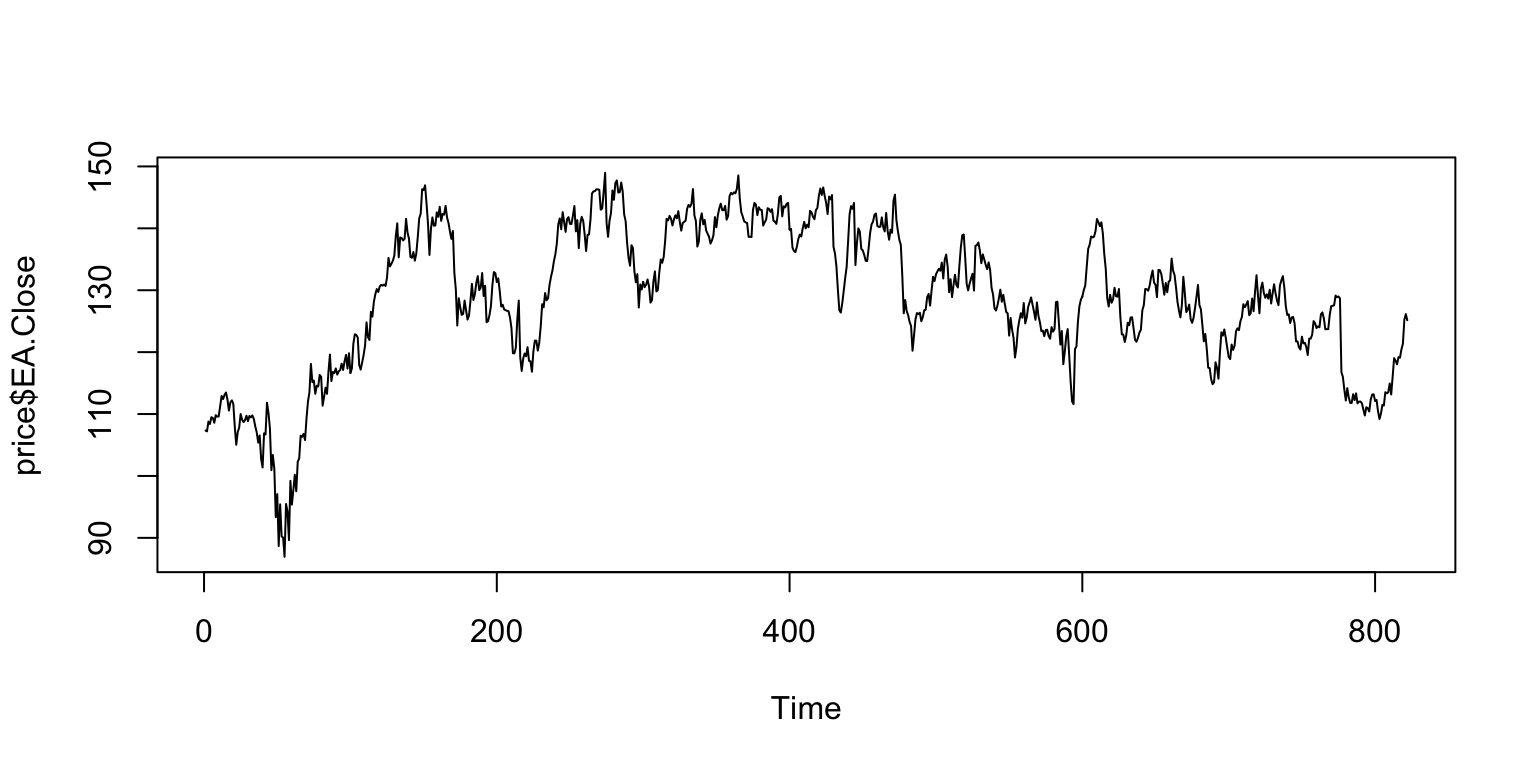
You can do a quick, simple plot with plot.ts(). Note that in this case the x-axis is the numerical index of the data point, and doesn’t show the date.

plot.ts(price$EA.Close)

Dygraphs

The dygraphs package offers flexibility and interactivity for time series.

• easily show multiple metrics at once.
• scroll over to see details.
• select chart area to zoom in.

library(dygraphs)
dygraph(price[,1:4], width='100%')

• subset for individual columns.
• easily add annotations for events.

## use dyEvent to add annotations
graph <- dygraph(price$EA.Close, width='100%')
graph <- dyEvent(graph, "2020-02-21","Start of Covid 19", labelLoc = 'top')
graph <- dyEvent(graph, "2021-06-10","New product announcements", labelLoc = 'top')
## print chart
graph

Decomposition Plots

Decomposition of a time series enables you to view it broken out into 3 key components (in addition to observed values):

• overall trend
• seasonality trending
• randomness trend (noise)

This can make it easier to ‘separate the signal from the noise’ and get a clearer sense of what is going on.

There has to be data over a long enough period to assess any seasonal trend, so this requires:

• frequency > 1, where 1=annual data; typically it would be at least 4 (quarterly), 12 (monthly), 52 (weekly), 365 (daily).
• period longer than 2 years: one year is not enough to establish a seasonal pattern over time.
  • if you get ‘Error in decomposet(): time series has no or less than 2 periods’ it is usually due to violating one or both of the above conditions.
• need to translate xts object to ts for this.

## Air Passengers has enough data
ap_decomp <- decompose(AirPassengers)
plot(ap_decomp)

apx_decomp <- decompose(ts(Air_xts, frequency=12))
plot(apx_decomp)

• same results with both approaches, although the original ts object maintains dates on x-axis, making it easier to interpret.
• interpretation: steady upward trend; peaks at mid-year; randomness fairly large at first, settles down, then appears to be growing over time.
• coincides with what we see in the observed data but makes the patterns more evident.

If we fetch some longer daily data for stock price, we can do the same:

## fetch some longer price data
price_d <- getSymbols('EA', from='2016-01-01', to='2021-12-31', auto.assign = FALSE)
price_decomp <- decompose(ts(price_d$EA.Close, frequency=365), type="additive")
plot(price_decomp)

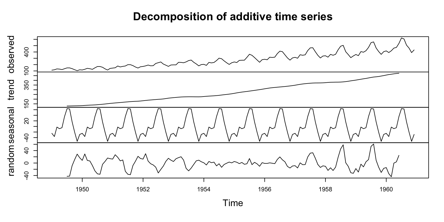
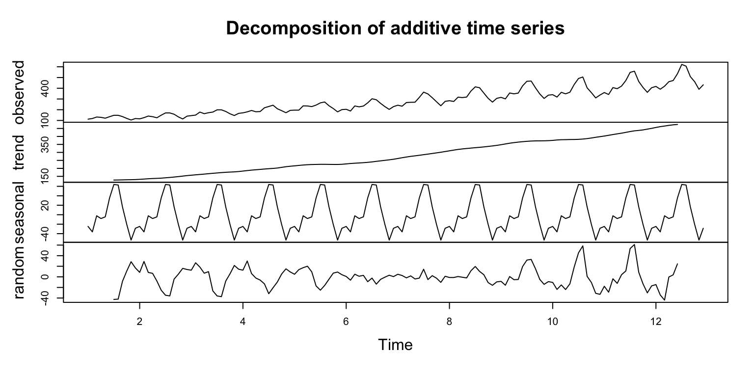
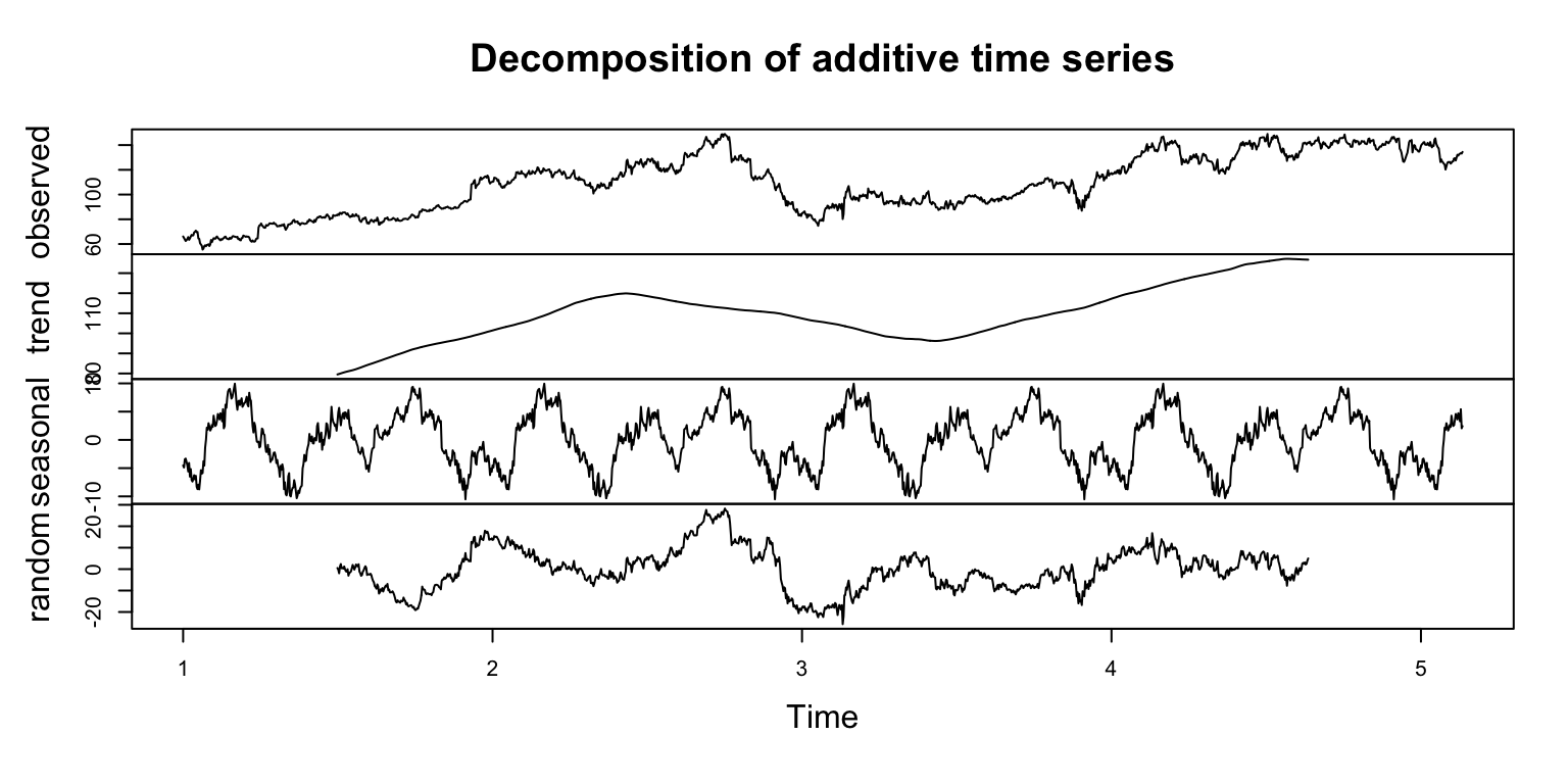
• we provide 6 full years of data and most of that is used to calculated decomposition.
• x-axis is year number.
• TREND: trending up to about half-way through year 2, then down until about the same point in year 3, then back up, looking like a peak in mid year 4. Not willing to stretch out beyond that. ;)
• SEASONAL: pattern has been detected where tends to be a dip at beginning of year, rising up to a peak toward end of first quarter, dropping sharply, smaller peak mid-year, peak in q3 or early q4, drop with a smaller bump at end of year.
• RANDOM: as to be expected with stock price in general, lots of randomness involved!

Looks like there may be money to be made riding the seasonal wave! Please: do not buy or sell stocks based on this information. ;)

Forecasting

A primary use case for time series objects is forecasting. This is a whole other, involved topic way beyond the scope of this post.

Here is a quick example to show how easy forecasting can be in R. Note that we need to bring in the forecast package for this. (There is also the amazing [tidyverts eco-system](https://tidyverts.org/) for working with time series that I have recently discovered - again, a whole other topic for another time.)

Get an ARIMA Model

Some basic terms, over-simplified for our purposes here:

• ARIMA stands for Auto Regression Integrated Moving Average
• One of the most widely-used time series forecasting methods, although certainly not the only.
• 3 essential parameters for ARIMA are p,d,q: p=periods of lag, d=differencing, q=error of the model.

library(forecast)
## get closing prices for forecasting
price_cl <- price[,4]
## get a model for the time series - using auto.arima for simplicity
fitA <- auto.arima(price_cl, seasonal=FALSE) ## can add trace=TRUE to see comparison of different models 
## show model
fitA

Series: price_cl 
ARIMA(0,1,0) 

sigma^2 = 5.11:  log likelihood = -1834
AIC=3671   AICc=3671   BIC=3675

The model we get back is ARIMA(0,1,1) which means p=0, d=1, q=1. We can generate a model by setting these parameters manually, but auto.arima automatically checks a variety of models and selects the best. When comparing models, lowest AIC and BIC are preferred.

We can check the accuracy of the model. Most useful item here for interpretation and comparison is MAPE (mean average percent error). In this case,

## check accuracy - based on historical data
accuracy(fitA)

                 ME RMSE  MAE     MPE MAPE  MASE    ACF1
Training set 0.0218 2.26 1.67 0.00169 1.33 0.999 -0.0405

fitAa <- accuracy(fitA)
100-fitAa[,5]

[1] 98.7

So in this case a MAPE of 1.325 can be seen as accuracy of 98.675%.

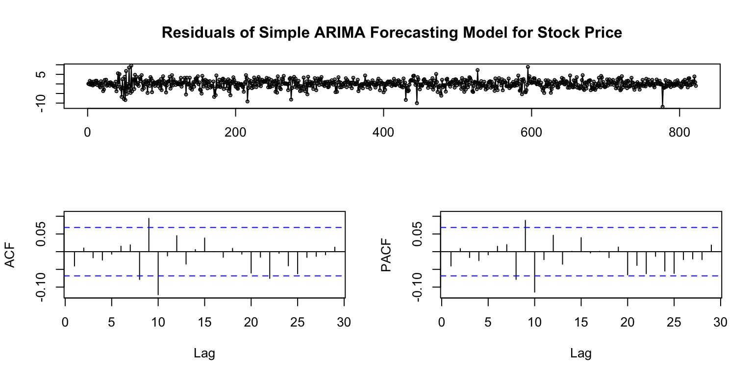
We can also plot the residuals of the model for visual inspection.

## check residuals
tsdisplay(residuals(fitA), main='Residuals of Simple ARIMA Forecasting Model for Stock Price')

As usual with residuals, we are looking for mean around 0, roughly evenly distributed. For ARIMA we also get ACF and PACF, where we are looking for bars to be short and at least within blue dotted lines. So looks like we are good to go here.

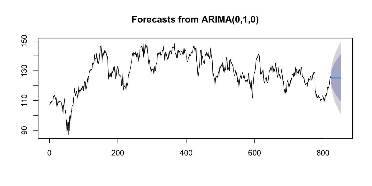
Create A Forecast

We just need a little more code to create and plot forecast. We can set the forecast period for whatever we want, based on the periodicity of the data, in this case days and we are looking out 30 days.

days=30
fcastA <- forecast(fitA, h=days)
plot(fcastA)

That was easy! And we can use this approach to quickly iterate over various models, if we are not convinced that auto.arima is the best. Of course you can use data frames to create forecasts of various sorts but the xts object makes it super-easy to apply common time series methods.

This also reveals a shortcoming of times-series forecasting:

• dependence of pattern recognition and pattern repetition, which can lead to conservative forecast, especially with noisy data.
• as a result, the forecast is: ‘steady as she goes, with possibility of moving either quite a bit higher or quite a bit lower’.

So not that useful. To be fair, if stock market prices are not actually predictable, so it is a perfectly reasonable outcome that grounds us in reality.

Conclusion

Times series objects are obviously a powerful way to work with time-based data and a go-to when your data is based on time. Particular strengths inculde:

• Ease of manipulation such as aggregation by date periods, selecting date ranges, period calculations.
• Some great visualization options for exploring the data.
• Forecasting which is really the bread and butter of time series objects.

There are some cases where you may prefer to stick with data frames:

• Multi-dimensional data: time series work best when each row represents a distinct time. If you are dealing with multi-dimensional data where dates are broken down by customer, or region, etc., especially in tidy format, you may want to stick with data frame.
• Visualization preferences: if you are more comfortable with using ggplot2 (or other visualization tools geared toward data frames) a data frame may be preferable. Or if the document you are producing has ggplot2 charts, you may want to maintain standard presentation.
• Forecasting needs: if you are doing time series forecasting you will want to use a time series object. If you’re not doing forecasting, there is less of a need. Limitation is that time series forecasting is based only on historical trends in the data and doesn’t include things like correlation with other factors.

Ultimately, the right tool for the job depends on a variety of situational factors, and having a collection of tools at your disposal helps you avoid the ‘when you have is a hammer…’ pitfall. If your data is based on time, time series should be in consideration.

So that’s quite a lot for one blog post - hopefully helps you make the most of your ‘time’!

Resources

Additional resources that may be helpful with time-series and xts in particular:

• xts Cheat Sheet.
• supplementary info. to cheat sheet.
• xts package vignette.
• time series section in R Cookbook 2nd Edition.
• tsibble package info. - time series for tidyverse.